3 Statistical Learning
Statistical Learning is also known as Machine learning(ML) in general. Here we try to develop ML methods to model/predict the occurrence of diabetic outcome.
3.1 Data Preprocessing
The data consists of different features that are needed to be mapped to a common reference frame. This is done by data preprocessing step.
library(caret) # ML package for various methods

# Create the training and test datasets
set.seed(100)
hci<-diab

# Step 1: Get row numbers for the training data
trainRowNumbers <- createDataPartition(hci$Outcome, p=0.8, list=FALSE) # Data partition for dividing the dataset into training and testing data set. This is useful for cross validation

# Step 2: Create the training  dataset
trainData <- hci[trainRowNumbers,]

# Step 3: Create the test dataset
testData <- hci[-trainRowNumbers,]

# Store X and Y for later use.
x = trainData[, 1:8]
y=trainData$Outcome

xt= testData[, 1:8]
yt=testData$Outcome
# # See the structure of the new dataset
3.2 Normalization of features
The features are normalized to a range of [0,1] using preproces command and using range method
preProcess_range_modeltr <- preProcess(trainData, method='range')
preProcess_range_modelts <- preProcess(testData, method='range')

trainData <- predict(preProcess_range_modeltr, newdata = trainData)
testData <- predict(preProcess_range_modelts, newdata = testData)

# Append the Y variable
trainData$Outcome <- y
testData$Outcome<-yt
levels(trainData$Outcome) <- c("Class0", "Class1") # Convert binary outcome into character for caret package
levels(testData$Outcome) <- c("Class0", "Class1")

#apply(trainData[, 1:8], 2, FUN=function(x){c('min'=min(x), 'max'=max(x))})
#str(trainData)
3.3 Options for training process
#fit control
fitControl <- trainControl(
  method = 'cv',                   # k-fold cross validation
  number = 5,                      # number of folds
  savePredictions = 'final',       # saves predictions for optimal tuning parameter
  classProbs = T,                  # should class probabilities be returned
  summaryFunction=twoClassSummary  # results summary function
)
3.4 Classical ML Models
The ML models we have chosen are: LDA, KNN, SVM, RandomForest, Adaboost. The Caret package provides a uniform program interface for all the machine models defined in the library.
# Step 1: Tune hyper parameters by setting tuneLength
set.seed(100)
model1 = train(Outcome ~ ., data=trainData, method='lda', tuneLength = 5, metric='ROC', trControl = fitControl)

model2 = train(Outcome ~ ., data=trainData, method='knn', tuneLength=2, trControl = fitControl)#KNN Model
model3 = train(Outcome ~ ., data=trainData, method='svmRadial', tuneLength=2, trControl = fitControl)#SVM
model4 = train(Outcome ~ ., data=trainData, method='rpart', tuneLength=2, trControl = fitControl)#RandomForest
model5 = train(Outcome ~ ., data=trainData, method='adaboost', tuneLength=2, trControl = fitControl) # Adaboost

# Compare model performances using resample()
models_compare <- resamples(list(LDA=model1,KNN=model2,SVM=model3,RF=model4, ADA=model5))

# Summary of the models performances
summary(models_compare)
##
## Call:
## summary.resamples(object = models_compare)
##
## Models: LDA, KNN, SVM, RF, ADA
## Number of resamples: 5
##
## ROC
## Min. 1st Qu. Median Mean 3rd Qu. Max. NA's
## LDA 0.8084302 0.8095930 0.8186047 0.8225000 0.8290698 0.8468023 0
## KNN 0.7332849 0.7409884 0.7819767 0.7731395 0.7904070 0.8190407 0
## SVM 0.7781977 0.8191860 0.8287791 0.8241860 0.8348837 0.8598837 0
## RF 0.6415698 0.6619186 0.7068314 0.7105233 0.7531977 0.7890988 0
## ADA 0.7741279 0.7752907 0.7796512 0.7942442 0.8098837 0.8322674 0
##
## Sens
## Min. 1st Qu. Median Mean 3rd Qu. Max. NA's
## LDA 0.8375 0.8625 0.8750 0.8725 0.8875 0.9000 0
## KNN 0.7750 0.7875 0.8375 0.8325 0.8625 0.9000 0
## SVM 0.8000 0.8375 0.8500 0.8550 0.8875 0.9000 0
## RF 0.7250 0.7625 0.7875 0.8100 0.8500 0.9250 0
## ADA 0.7250 0.7875 0.8125 0.8075 0.8500 0.8625 0
##
## Spec
## Min. 1st Qu. Median Mean 3rd Qu. Max. NA's
## LDA 0.4651163 0.5348837 0.5813953 0.5534884 0.5813953 0.6046512 0
## KNN 0.3488372 0.4883721 0.4883721 0.4837209 0.5348837 0.5581395 0
## SVM 0.4651163 0.5116279 0.5116279 0.5488372 0.5813953 0.6744186 0
## RF 0.4186047 0.5581395 0.5813953 0.6000000 0.6511628 0.7906977 0
## ADA 0.5581395 0.5813953 0.6279070 0.6139535 0.6279070 0.6744186 0# Draw box plots to compare models
scales <- list(x=list(relation="free"), y=list(relation="free"))
bwplot(models_compare, scales=scales)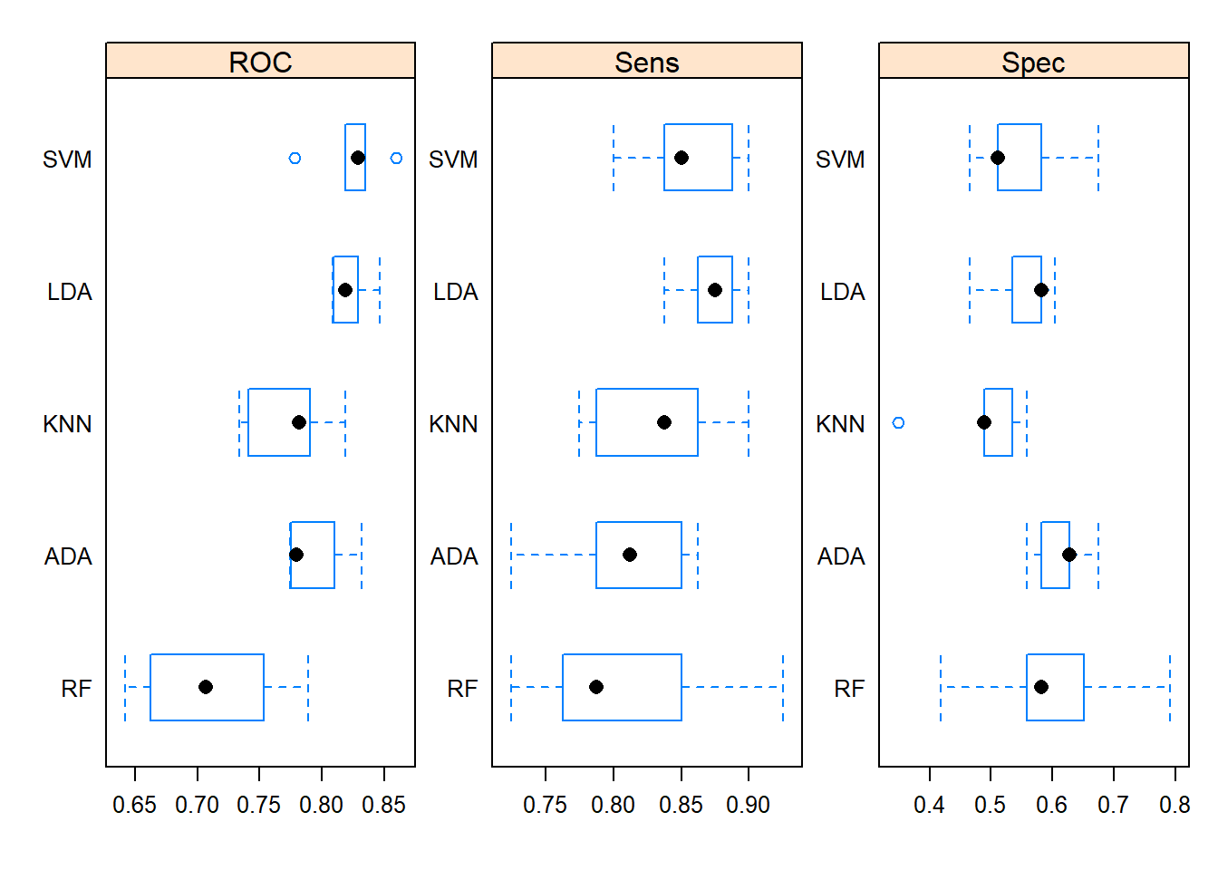
3.5 Testing the performance for the test data set.
# Step 2: Predict on testData and Compute the confusion matrix
# Using LDA Model
predicted <- predict(model1, testData[,1:8])
confusionMatrix(reference = testData$Outcome, data = predicted, mode='everything')
## Confusion Matrix and Statistics
##
## Reference
## Prediction Class0 Class1
## Class0 48 5
## Class1 52 48
##
## Accuracy : 0.6275
## 95% CI : (0.5457, 0.7042)
## No Information Rate : 0.6536
## P-Value [Acc > NIR] : 0.7788
##
## Kappa : 0.3192
## Mcnemar's Test P-Value : 1.109e-09
##
## Sensitivity : 0.4800
## Specificity : 0.9057
## Pos Pred Value : 0.9057
## Neg Pred Value : 0.4800
## Precision : 0.9057
## Recall : 0.4800
## F1 : 0.6275
## Prevalence : 0.6536
## Detection Rate : 0.3137
## Detection Prevalence : 0.3464
## Balanced Accuracy : 0.6928
##
## 'Positive' Class : Class0
##