Chapter 1 Introduction

Malaria is a deadly disease predominantly caused by a parasite name Plasmodium falciparum which is transmitted by mosquito. It shows symptoms such as high fever and chills, which not treated in due time can be fatal. The disease is diagnosed by capturing the cell images of the blood and the presence of parasitic stains can be used to detect the Malarial disease.

1.1 Dataset

The Kaggle dataset consists of two folders namely uninfected and parasitized cell images. The images are color images which are resized to a dimension of \[128 \times 128\]. The original dataset provides a total of around 25000 images. However, for running our simple DL algorithm we will be using only 100 images for each class.

1.2 Python Programming ENV

The following section explains about different Python Libraries we would be using for our Malaria detection method. As we are doing the development in the Google Colab, we don’t need to install any module here. It is alreadly configured in the Colab ENV, only we have to import the required libraries for our application. The Python codes is grouped into different code chunks for each understanding.

1.2.1 Importing of common array and plotting librariers

This is for data importing and manipulation using NUMPY and PANDAS. Matplotlib and Seaborn for plotting graphs and images.

import numpy as np
import pandas as pd
import matplotlib.pyplot as plt
from matplotlib import style
import seaborn as sns

1.2.2 Importing of OpenCV and Scikit-learn

OpenCV and Scikit-learn for image processing and machine learning respectivley.

import cv2 
import os
from sklearn.feature_extraction import image

1.3 Data Preprocessing

Here we initialize a set of lists X & Z for the images and the labels.

from tqdm import tqdm
X=[]
Z=[]
IMG_SIZE=128
norm_DIR='data/uninfected'
mal_DIR='data/parasitized'

1.3.1 Creation of lists for the images and the labels

Here we create two functions for creating image lists and labels.

def assign_label(img,ret_type):
    return ret_type

def make_train_data(ret_type,DIR):
    for img in tqdm(os.listdir(DIR)):
        label=assign_label(img,ret_type)
        path = os.path.join(DIR,img)
        img = cv2.imread(path,cv2.IMREAD_COLOR)
        img = cv2.resize(img, (IMG_SIZE,IMG_SIZE))
        
        X.append(np.array(img))
        Z.append(str(label))
    

Here we call the functions to perform the array formation for the images and the labels.

make_train_data('Uninfected',norm_DIR)

## 
  0%|          | 0/100 [00:00<?, ?it/s]
100%|##########| 100/100 [00:00<00:00, 1217.99it/s]

print(len(X))

## 100

make_train_data('Parasitized',mal_DIR)

## 
  0%|          | 0/100 [00:00<?, ?it/s]
100%|##########| 100/100 [00:00<00:00, 1520.84it/s]

print(len(X))

## 200

1.4 Plotting of the sample images

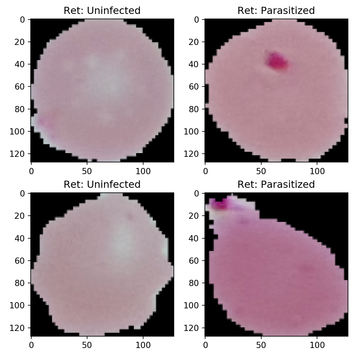
Here we plot some of the cell images of malarial and uninfected person blood.

import random as rn
fig,ax=plt.subplots(2,2)
fig.set_size_inches(6,6)
for i in range(2):
    for j in range (2):
        l=rn.randint(0,len(Z))
        ax[i,j].imshow(X[l])
        ax[i,j].set_title('Ret: '+Z[l])
        plt.tight_layout()
        

## Label Encoding Here is a label preprocessing where we perform one hot encoding of the labels.

from sklearn.preprocessing import LabelEncoder
import tensorflow 
from tensorflow.keras.utils import to_categorical

le=LabelEncoder()
Y=le.fit_transform(Z)
Y=to_categorical(Y,2)
X=np.array(X)
X=X/255

1.5 Data Splitting

Here we perform the splitting of the dataset into Training (75%) and Testing (25%) datasets.

from sklearn.model_selection import train_test_split
from sklearn.metrics import accuracy_score,precision_score,recall_score,confusion_matrix,roc_curve,roc_auc_score

x_train,x_test,y_train,y_test=train_test_split(X,Y,test_size=0.25,random_state=42)
print(x_train.shape)

## (150, 128, 128, 3)

print(y_train.shape)

## (150, 2)

print(x_test.shape)

## (50, 128, 128, 3)

print(y_test.shape)

## (50, 2)

1.6 Deep Learning Model based on CNN

This section explains about our deep learning model based on CNN. Here we will use 4 Convolutional blocks and 4 Max-Pooling blocks. Finally we will be having a classification layer based on SOFTMAX function for classifying the cell images as uninfected or parasitized.

# # modelling starts using a CNN.
from tensorflow.keras.models import Sequential
import tensorflow as tf

model = Sequential()
model.add(tf.keras.layers.Conv2D(filters = 32, kernel_size = (5,5),padding = 'Same',activation ='relu', input_shape = (128,128,3)))

## WARNING:tensorflow:From /home/rajumanj/anaconda3/envs/rajutf/lib/python3.7/site-packages/tensorflow_core/python/ops/resource_variable_ops.py:1630: calling BaseResourceVariable.__init__ (from tensorflow.python.ops.resource_variable_ops) with constraint is deprecated and will be removed in a future version.
## Instructions for updating:
## If using Keras pass *_constraint arguments to layers.

model.add(tf.keras.layers.MaxPooling2D(pool_size=(2,2)))


model.add(tf.keras.layers.Conv2D(filters = 64, kernel_size = (3,3),padding = 'Same',activation ='relu'))
model.add(tf.keras.layers.MaxPooling2D(pool_size=(2,2), strides=(2,2)))
 

model.add(tf.keras.layers.Conv2D(filters =96, kernel_size = (3,3),padding = 'Same',activation ='relu'))
model.add(tf.keras.layers.MaxPooling2D(pool_size=(2,2), strides=(2,2)))

model.add(tf.keras.layers.Conv2D(filters = 96, kernel_size = (3,3),padding = 'Same',activation ='relu'))
model.add(tf.keras.layers.MaxPooling2D(pool_size=(2,2), strides=(2,2)))

model.add(tf.keras.layers.Flatten())
model.add(tf.keras.layers.Dense(512,activation ='relu'))
model.add(tf.keras.layers.Dense(2, activation = "softmax"))

1.7 Deep learning model architecture

This sections shows the DL model based on CNN for cell image classification. The number of parametes are also provided here.

model.summary()

## Model: "sequential"
## _________________________________________________________________
## Layer (type)                 Output Shape              Param #   
## =================================================================
## conv2d (Conv2D)              (None, 128, 128, 32)      2432      
## _________________________________________________________________
## max_pooling2d (MaxPooling2D) (None, 64, 64, 32)        0         
## _________________________________________________________________
## conv2d_1 (Conv2D)            (None, 64, 64, 64)        18496     
## _________________________________________________________________
## max_pooling2d_1 (MaxPooling2 (None, 32, 32, 64)        0         
## _________________________________________________________________
## conv2d_2 (Conv2D)            (None, 32, 32, 96)        55392     
## _________________________________________________________________
## max_pooling2d_2 (MaxPooling2 (None, 16, 16, 96)        0         
## _________________________________________________________________
## conv2d_3 (Conv2D)            (None, 16, 16, 96)        83040     
## _________________________________________________________________
## max_pooling2d_3 (MaxPooling2 (None, 8, 8, 96)          0         
## _________________________________________________________________
## flatten (Flatten)            (None, 6144)              0         
## _________________________________________________________________
## dense (Dense)                (None, 512)               3146240   
## _________________________________________________________________
## dense_1 (Dense)              (None, 2)                 1026      
## =================================================================
## Total params: 3,306,626
## Trainable params: 3,306,626
## Non-trainable params: 0
## _________________________________________________________________

1.8 Model Compile

Here we compile the CNN model for checking any errors and initialize the ADAM optimizer. We have used Cross-Entropy has our loss function.

model.compile(optimizer=tf.keras.optimizers.Adam(lr=0.001),loss='categorical_crossentropy',metrics=['accuracy'])

1.9 Model Training

Here we train our DL model using FIT function. We use batch size of 4 and training epochs of 5

print('# Fit model on training data')

history = model.fit(x_train, y_train,
                    batch_size=4,
                    epochs=10,
                    # We pass some validation for
                    # monitoring validation loss and metrics
                    # at the end of each epoch
                    validation_data=(x_test, y_test))
                    

1.10 Plotting Variables of Training Sequence

print(history.history.keys())

## dict_keys(['loss', 'acc', 'val_loss', 'val_acc'])

1.11 Training Sequence-Accuracy

The plot showing the accuracy of the DL model during training and testing phase.

# summarize history for accuracy
plt.rcParams["figure.dpi"] = 200
plt.rcParams["figure.figsize"] = (4,3)
plt.plot(history.history['acc'])
plt.plot(history.history['val_acc'])
plt.title('model accuracy')
plt.ylabel('accuracy')
plt.xlabel('epoch')
plt.xlim([min(plt.ylim()),10])

## (0.4380000099539757, 10)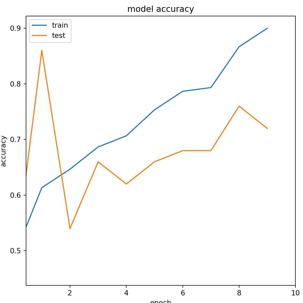

plt.legend(['train', 'test'], loc='upper left')
plt.show()

1.12 Training Sequence-Loss Function

The plot showing the loss of the DL model during training and testing phase.

# summarize history for loss
plt.plot(history.history['loss'])
plt.plot(history.history['val_loss'])
plt.rcParams["figure.figsize"] = (4,3)

plt.title('model loss')
plt.ylabel('loss')
plt.xlabel('epoch')
plt.xlim([min(plt.ylim()),10])

## (0.2958974132724106, 10)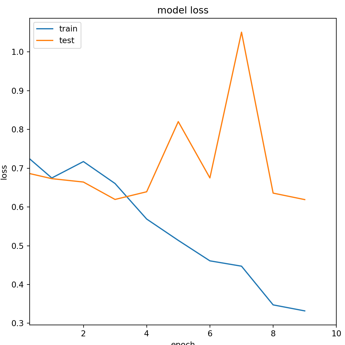

plt.legend(['train', 'test'], loc='upper left')
plt.show()

1.13 Model Prediction for Evaluation

predictions = model.predict(x_test)
predicted_classes = np.argmax(predictions, axis=1)
true_classes=np.argmax(y_test,axis=1)

1.14 Testing Accuracy and Confusion Matrix

import sklearn.metrics as metrics
from sklearn.metrics import confusion_matrix
print('Accuracy for malaria disease classifier=',metrics.accuracy_score(predicted_classes,true_classes))

## Accuracy for malaria disease classifier= 0.72

print('Confusion matrix=\n',confusion_matrix(true_classes, predicted_classes))

## Confusion matrix=
##  [[16  7]
##  [ 7 20]]

1.15 ROC plot of the DL model

from sklearn.metrics import roc_curve, auc
fpr_keras, tpr_keras, thresholds_keras = roc_curve(true_classes, predictions[:,1])
auc_rf = auc(fpr_keras, tpr_keras)
auc_rf

## 0.8083735909822867

plt.rcParams["figure.figsize"] = (4,3)
plt.figure(1)
plt.plot([0, 1], [0, 1], 'k--')
plt.plot(fpr_keras, tpr_keras, label='ROC (area = {:.3f})'.format(auc_rf))
plt.xlabel('False positive rate')
plt.ylabel('True positive rate')
plt.title('ROC curve')
plt.legend(loc='best')
plt.show()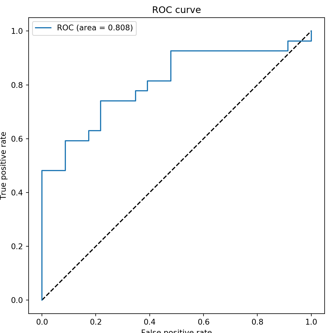

Some papers for related information on Deep Learning Technologies:

• (Bhandary et al. 2020)
• (Lakshmi, Thanaraj, and Arunmozhi 2019)
• (Xie 2015)

References

Bhandary, Abhir, G Ananth Prabhu, V Rajinikanth, K Palani Thanaraj, Suresh Chandra Satapathy, David E Robbins, Charles Shasky, Yu-Dong Zhang, João Manuel RS Tavares, and N Sri Madhava Raja. 2020. “Deep-Learning Framework to Detect Lung Abnormality–a Study with Chest X-Ray and Lung Ct Scan Images.” Pattern Recognition Letters 129. Elsevier: 271–78.

Lakshmi, D, K Palani Thanaraj, and M Arunmozhi. 2019. “Convolutional Neural Network in the Detection of Lung Carcinoma Using Transfer Learning Approach.” International Journal of Imaging Systems and Technology. Wiley Online Library.

Xie, Yihui. 2015. Dynamic Documents with R and Knitr. 2nd ed. Boca Raton, Florida: Chapman; Hall/CRC. http://yihui.org/knitr/.